Iterative Solve: CG, LSMR, and Polynomial Preconditioning

This example demonstrates the solve() method exposed on every PyGROG operator (SparseFFT, MaskedFFT and their pygrog.gadgets decorators), and the pygrog.PolynomialPreconditioner accelerator.

The pipeline mirrors Basic Usage: mri-nufft Baseline vs PyGROG:

1. Simulate non-Cartesian k-space from a BrainWeb phantom.

2. GROG-grid into Cartesian space (sparse and dense paths).

3. Solve the regularised least-squares problem

   \[\hat x \;=\; \arg\min_x \; \| A x - b \|_2^2 + \lambda^2 \| x \|_2^2\]

   using pygrog.cg(), pygrog.lsmr(), and a polynomial- preconditioned pygrog.cg().

import matplotlib.pyplot as plt
import numpy as np
from brainweb_dl import get_mri
from mrinufft import get_operator, initialize_2D_spiral
from mrinufft.density import voronoi

from pygrog import PolynomialPreconditioner
from pygrog.calib import GrogInterpolator
from pygrog.operator import MaskedFFT, SparseFFT

image = get_mri(0, "T1")

nufft = get_operator("finufft")(

/home/docs/checkouts/readthedocs.org/user_builds/pygrog/envs/latest/lib/python3.12/site-packages/mrinufft/_utils.py:67: UserWarning: Samples will be rescaled to [-pi, pi), assuming they were in [-0.5, 0.5)
  warnings.warn(
k-space shape: (16, 28800)

GROG calibration and gridding

Set up GrogInterpolator to grid the non-Cartesian k-space onto Cartesian samples. Prepare both a sparse path and a dense (gridded) path for comparison.

calib = nufft.adj_op(kspace_nc)  # quick low-res-ish phantom estimate
calib = calib.astype(np.complex64, copy=False)[None]  # (1, *shape)

grog = GrogInterpolator(
    shape=shape,
    coords=samples.reshape(48, 600, 2),
    kernel_width=2,
    oversamp=2.0,
    image_shape=shape,
)

calib_full = smaps * image.astype(
    np.complex64
)  # (n_coils, *shape) — ground-truth coil images


grog.calc_interp_table(calib_full, lamda=0.01, precision=1)

kspace_nc_shaped = kspace_nc.reshape(n_coils, 48, 600)

# Sparse path
sparse = grog.interpolate(kspace_nc_shaped, ret_image=False)
op_sp = SparseFFT(plan=grog.plan, smaps=smaps)
b_sp = sparse * np.asarray(grog.plan.pre_weights)
b_sp = b_sp.reshape(*b_sp.shape[:-1], *op_sp.natural_shape)

# Dense/grid path
kgrid, mplan = grog.interpolate(kspace_nc_shaped, grid=True)
op_m = MaskedFFT(plan=mplan, smaps=smaps)
b_m = kgrid

Conjugate Gradient (CG) Solver

Solve the regularized normal equations using CG. PyGROG operators automatically dispatch to CG when Toeplitz acceleration is available.

residuals_cg = []


img_cg = op_m.solve(
    b_m,
    method="cg",
    max_iter=20,
    damp=1e-3,
    callback=_cb_cg,
)
print(f"CG: {len(residuals_cg)} iterations")

CG: 20 iterations

LSMR Solver

Use LSMR (iterative solver for regularised least-squares) as an alternative to CG for comparison.

img_lsmr = op_m.solve(
    b_m,
    method="lsmr",
    max_iter=20,
    callback=_cb_lsmr,
)
print(f"LSMR: {len(residuals_lsmr)} iterations")

LSMR: 20 iterations

Polynomial Preconditioned CG (PCG)

pygrog.PolynomialPreconditioner builds a polynomial approximation to the inverse of A^H A from Chebyshev polynomials. Each application requires degree matrix-vector products but typically accelerates CG convergence significantly.

pc = PolynomialPreconditioner(op_m, degree=3, n_power_iter=10)
print(f"Preconditioner spectrum estimate: {pc.spectrum}")
print(f"Polynomial coefficients: {pc.coeffs}")

img_pcg = op_m.solve(
    b_m,
    method="cg",
    max_iter=20,
    damp=1e-3,
    preconditioner=pc,
    callback=_cb_pcg,
)
print(f"PCG: {len(residuals_pcg)} iterations")

Preconditioner spectrum estimate: (0.0, 1.0315111130475998)
Polynomial coefficients: [11.633418048712429, -39.47312118639093, 51.02303560548171, -22.25896137426571]
PCG: 20 iterations

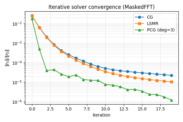
Compare convergence

fig, ax = plt.subplots(figsize=(6, 4))

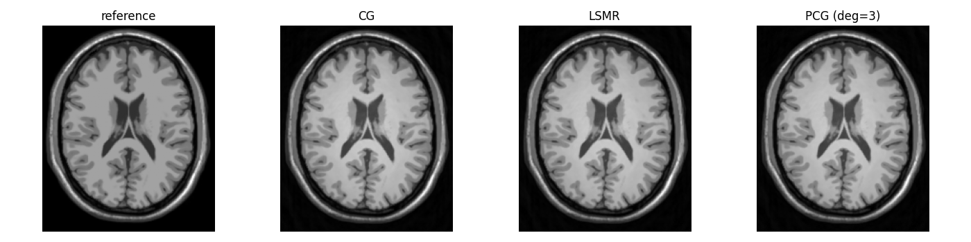
Visualise the reconstructions

fig, axes = plt.subplots(1, 4, figsize=(14, 3.5))

The same solve() API works on the sparse path

img_cg_sp = op_sp.solve(b_sp, method="cg", max_iter=20, damp=1e-3)
print(
    "SparseFFT solve image shape:",
    tuple(img_cg_sp.shape),
)

SparseFFT solve image shape: (217, 181)