Utils Tour: Coil Compression and NLINV

This example introduces two utility routines from pygrog.utils:

1. Coil compression (coil_compress()) — reduces the number of receiver coils via PCA to speed up downstream processing without significant SNR loss.

2. NLINV coil calibration (nlinv_calib()) — estimates coil sensitivity maps from undersampled k-space data using the nonlinear-inverse (NLINV) algorithm.

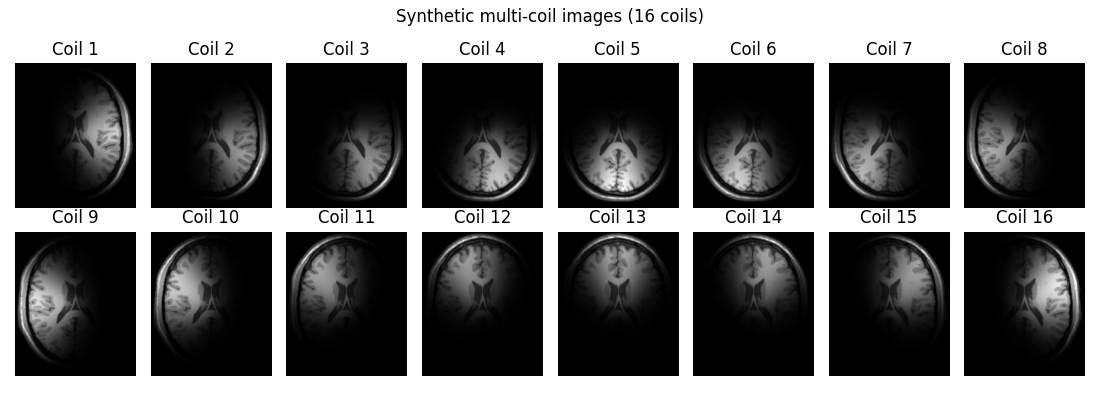
All data use a BrainWeb T1-weighted phantom: a multi-coil dataset is constructed by multiplying it with synthetic coil sensitivity maps.

import matplotlib.colors as mcolors
import matplotlib.pyplot as plt
import numpy as np
import torch



from brainweb_dl import get_mri



image = get_mri(0, "T1")

Coil images shape: (16, 217, 181)
K-space shape    : (16, 217, 181)

fig, axes = plt.subplots(2, n_coils // 2, figsize=(11, 4))

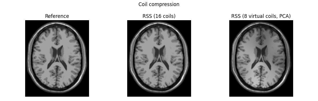
Coil Compression via PCA

Use coil_compress() to reduce the number of receiver coils via PCA on k-space data, reducing computational cost with minimal SNR loss. The function returns the compressed k-space and the compression matrix W of shape (n_virtual, n_coils).

# Prepare k-space data for compression
kspace_flat = kspace_full.reshape(n_coils, -1)  # (n_coils, n_samples)

n_virtual = 8


from pygrog.utils import coil_compress

kspace_cc, W = coil_compress(kspace_flat, n_virtual)

print(f"\nOriginal coils   : {kspace_flat.shape[0]}")
print(f"Virtual coils    : {kspace_cc.shape[0]}")
print(f"Compression matrix: {W.shape}")

# Reconstruct coil images from compressed data
kspace_cc_full = kspace_cc.reshape(n_virtual, *image_shape)
coil_images_cc = np.fft.fftshift(
    np.fft.ifft2(np.fft.ifftshift(kspace_cc_full, axes=(-2, -1))), axes=(-2, -1)
)

# RSS of compressed coils vs original
rss_orig = np.sqrt((np.abs(coil_images) ** 2).sum(0))
rss_cc = np.sqrt((np.abs(coil_images_cc) ** 2).sum(0))

Original coils   : 16
Virtual coils    : 8
Compression matrix: (8, 16)

fig, axes = plt.subplots(1, 3, figsize=(11, 3.5))

Note

Coil compression is lossless when n_coils >= original_n_coils and near-lossless when the retained energy fraction is high (e.g. > 0.99). Use a float threshold coil_compress(data, 0.99) for automatic rank selection.

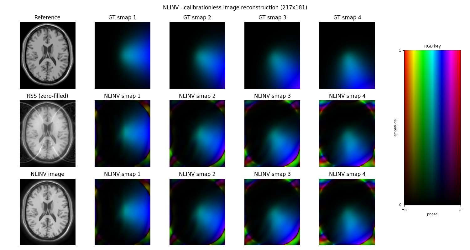
NLINV Sensitivity Estimation

nlinv_calib() estimates coil sensitivity maps jointly with the image using the nonlinear-inverse (NLINV) algorithm (Uecker et al.2008). It requires a small fully-sampled ACS centre to bootstrap, but no explicit prior knowledge of the sensitivity maps.

The function supports two modes: * ``cal_width=None`` - full k-space calibrationless reconstruction * ``cal_width=24`` - fast calibration mode with central k-space cropping

from pygrog.utils import nlinv_calib

acs = 8  # fully-sampled ACS centre width (columns), as in MATLAB reference
cal_width = 24  # NLINV internal calibration resolution for Step 2

# Cartesian undersampling mask: R=2 readout subsampling + 8-col ACS centre
mask = np.zeros(image_shape, dtype=bool)
mask[:, ::2] = True  # R=2 subsampling on readout (column) direction
cx = image_shape[1] // 2
cy = image_shape[0] // 2
mask[cy - acs // 2 : cy + acs // 2, cx - acs // 2 : cx + acs // 2] = True  # ACS

kspace_us = kspace_full * mask[np.newaxis]

print(f"\nUndersampling factor : {mask.size / mask.sum():.2f}x")
print(f"ACS region           : all rows x {acs} cols")
print(f"Undersampled k-space : {kspace_us.shape}")

ncols_show = min(n_coils // 2, 4)

# Zero-filled RSS image from undersampled data (baseline)
coil_images_us = np.fft.fftshift(
    np.fft.ifft2(np.fft.ifftshift(kspace_us, axes=(-2, -1))), axes=(-2, -1)
)
rss_us = np.sqrt((np.abs(coil_images_us) ** 2).sum(0))

Undersampling factor : 1.99x
ACS region           : all rows x 8 cols
Undersampled k-space : (16, 217, 181)

NLINV Step 1: Full k-space calibrationless reconstruction

Call nlinv_calib() with cal_width=None to solve jointly for image and sensitivity maps using the entire undersampled k-space. cal_width=None -> full k-space, no cropping, matching MATLAB reference

smaps_full, _, image_full = nlinv_calib(
    kspace_us,
    cal_width=None,
    ndim=2,
    mask=mask,
    ret_cal=True,
    ret_image=True,
)

smaps_full_np = (
    smaps_full.numpy() if isinstance(smaps_full, torch.Tensor) else smaps_full
)
image_full_np = (
    image_full.numpy() if isinstance(image_full, torch.Tensor) else image_full
)

print(f"\n[Step 1] Smaps shape     : {smaps_full_np.shape}")
print(f"[Step 1] NLINV image shape: {image_full_np.shape}")

[Step 1] Smaps shape     : (16, 217, 181)
[Step 1] NLINV image shape: (217, 181)

fig, axes = plt.subplots(3, ncols_show + 1, figsize=(3 * (ncols_show + 1), 8))

NLINV Step 2: Calibration mode with central k-space cropping

Call nlinv_calib() with cal_width=24 to crop to the central region and solve for low-resolution sensitivity maps and a synthesized calibration k-space patch (useful for GRAPPA/GROG training).

smaps_cal, grappa_train, image_cal = nlinv_calib(
    kspace_us,
    cal_width=cal_width,
    ndim=2,
    mask=mask,
    ret_cal=True,
    ret_image=True,
)

smaps_cal_np = smaps_cal.numpy() if isinstance(smaps_cal, torch.Tensor) else smaps_cal
grappa_train_np = (
    grappa_train.numpy() if isinstance(grappa_train, torch.Tensor) else grappa_train
)
image_cal_np = image_cal.numpy() if isinstance(image_cal, torch.Tensor) else image_cal

print(f"\n[Step 2] Smaps shape       : {smaps_cal_np.shape}")
print(f"[Step 2] Low-res image shape: {image_cal_np.shape}")
print(f"[Step 2] Cal k-space shape  : {grappa_train_np.shape}")

[Step 2] Smaps shape       : (16, 217, 181)
[Step 2] Low-res image shape: (24, 24)
[Step 2] Cal k-space shape  : (16, 24, 24)

# Low-res image and smaps at cal_width resolution

fig, axes = plt.subplots(1, ncols_show + 1, figsize=(3 * (ncols_show + 1), 3))

# Zero-filled vs synthesized central k-space patch

acr_zf = kspace_us[

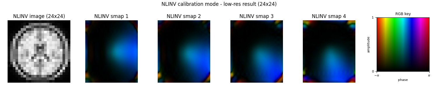
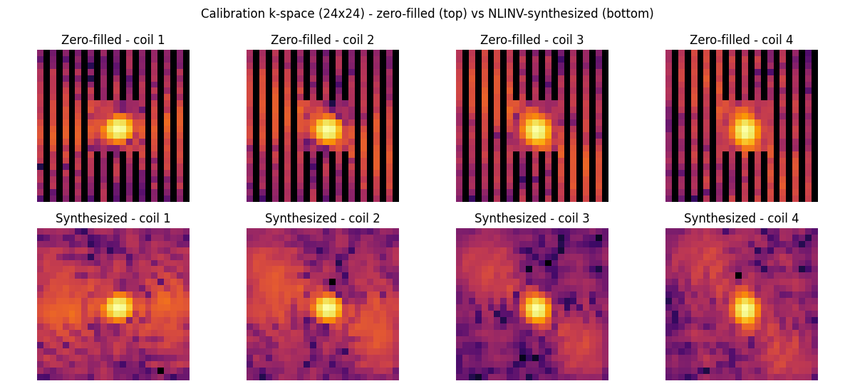
Note

In calibration mode (integer cal_width) the sensitivity maps are estimated at low resolution and zero-padded to the full FOV - they are smoother but less accurate near the FOV boundary. Use cal_width=None when full image reconstruction quality matters; use an integer cal_width when only the synthesized k-space patch and fast coil estimates are needed (e.g.as input to GROG/GRAPPA kernel training).

plt.show()

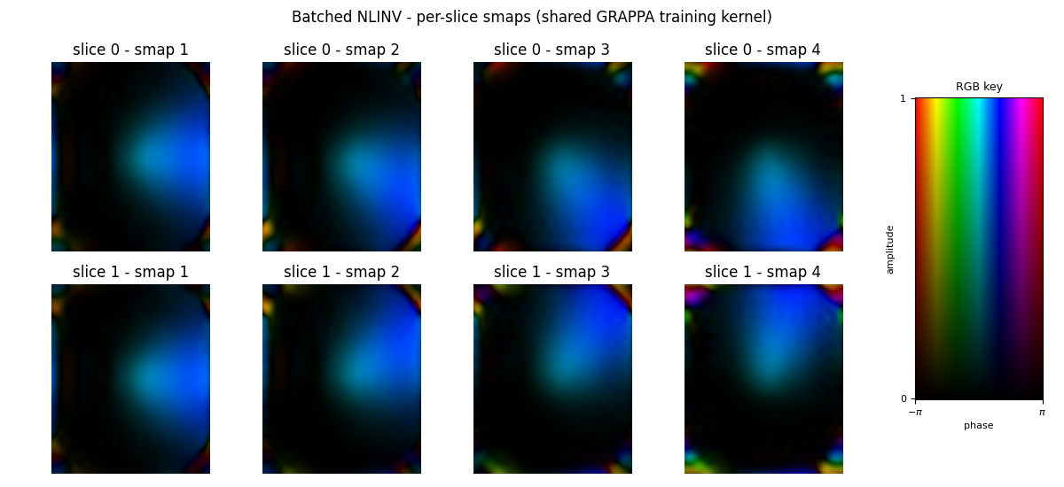
Multi-slice batched NLINV calibration

nlinv_calib() accepts a leading batch axis and runs the calibration once per batch element. Sensitivity maps and image reconstructions are returned per-slice; the synthesized GRAPPA training k-space can optionally be averaged across the batch with train_reduce='mean' to produce a single shared kernel.

batch_slices = np.stack([kspace_us, kspace_us[:, ::-1, :]], axis=0)
print(f"\n[Multi-slice] batched k-space shape : {batch_slices.shape}")

# Per-slice smaps + shared (mean-reduced) GRAPPA training k-space.
smaps_b, train_b_mean, image_b = nlinv_calib(
    batch_slices,
    cal_width=cal_width,
    ndim=2,
    ret_cal=True,
    ret_image=True,
    train_reduce="mean",
)
print(f"[Multi-slice] smaps shape           : {tuple(smaps_b.shape)}")
print(f"[Multi-slice] image shape           : {tuple(image_b.shape)}")
print(f"[Multi-slice] mean-train shape      : {tuple(train_b_mean.shape)}")

[Multi-slice] batched k-space shape : (2, 16, 217, 181)
[Multi-slice] smaps shape           : (2, 16, 217, 181)
[Multi-slice] image shape           : (2, 24, 24)
[Multi-slice] mean-train shape      : (16, 24, 24)

fig, axes = plt.subplots(2, ncols_show, figsize=(3 * ncols_show, 5.5))