Basic Usage: mri-nufft Baseline vs PyGROG

This example follows a realistic non-Cartesian pipeline:

1. Use brainweb-dl to load a brain phantom.

2. Use mri-nufft to generate the trajectory, sensitivity maps, non-Cartesian k-space data, and a reference adjoint reconstruction.

3. Use GrogInterpolator to grid and reconstruct, then compare PyGROG against the mri-nufft reference.

import matplotlib.pyplot as plt
import numpy as np

from brainweb_dl import get_mri

from mrinufft import get_operator, initialize_2D_spiral
from mrinufft.density import voronoi

from pygrog.calib import GrogInterpolator
from pygrog.operator import MaskedFFT, SparseFFT

image = get_mri(0, "T1")

Downloading T1+ICBM+normal+1mm+pn0+rf0: 0.00B [00:00, ?B/s]


Downloading T1+ICBM+normal+1mm+pn0+rf0: 1.00kB [00:00, 5.40kB/s]


Downloading T1+ICBM+normal+1mm+pn0+rf0: 192kB [00:00, 805kB/s]


Downloading T1+ICBM+normal+1mm+pn0+rf0: 1.27MB [00:00, 4.70MB/s]


Downloading T1+ICBM+normal+1mm+pn0+rf0: 2.28MB [00:00, 6.73MB/s]


Downloading T1+ICBM+normal+1mm+pn0+rf0: 3.27MB [00:00, 7.90MB/s]


Downloading T1+ICBM+normal+1mm+pn0+rf0: 4.19MB [00:00, 8.47MB/s]


Downloading T1+ICBM+normal+1mm+pn0+rf0: 5.09MB [00:00, 8.75MB/s]


Downloading T1+ICBM+normal+1mm+pn0+rf0: 5.96MB [00:00, 8.79MB/s]


Downloading T1+ICBM+normal+1mm+pn0+rf0: 6.82MB [00:01, 8.57MB/s]


Downloading T1+ICBM+normal+1mm+pn0+rf0: 7.66MB [00:01, 7.62MB/s]

smaps = _synthetic_smaps(shape, n_coils=n_coils)

/home/docs/checkouts/readthedocs.org/user_builds/pygrog/envs/latest/lib/python3.12/site-packages/mrinufft/_utils.py:67: UserWarning: Samples will be rescaled to [-pi, pi), assuming they were in [-0.5, 0.5)
  warnings.warn(
/home/docs/checkouts/readthedocs.org/user_builds/pygrog/envs/latest/lib/python3.12/site-packages/mrinufft/_utils.py:67: UserWarning: Samples will be rescaled to [-pi, pi), assuming they were in [-0.5, 0.5)
  warnings.warn(
k-space shape   : (16, 28800)
image shape     : (217, 181)

PyGROG calibration setup

First, prepare the calibration data and initialize the GROG interpolator. This is the setup phase — the actual API calls are shown in the next cells.

# Calibrate GROG from the 24x24 k-space centre of compressed coil images.
# Using the full k-space degrades GRAPPA conditioning; the low-frequency
# centre is all that is needed to estimate the GRAPPA operators.
coil_calib = smaps * image[None, ...]
calib_cart_full = np.fft.fftshift(
    np.fft.fftn(np.fft.ifftshift(coil_calib, axes=(-2, -1)), axes=(-2, -1)),
    axes=(-2, -1),
).astype(np.complex64)
calib_size = 24
cy, cx = shape[0] // 2, shape[1] // 2
calib_cart = calib_cart_full[
    :,
    cy - calib_size // 2 : cy + calib_size // 2,
    cx - calib_size // 2 : cx + calib_size // 2,
]

# mri-nufft coordinates are in [-0.5, 0.5): scale to PyGROG grid units.
coords = (samples * np.asarray(shape, dtype=np.float32)).astype(np.float32)

GROG Calibration

Initialize GrogInterpolator with the calibration region and compute the GRAPPA operators via FFT-based kernel estimation.

grog = GrogInterpolator(
    shape=shape, coords=coords, kernel_width=2, oversamp=1.25, image_shape=shape
)
grog.calc_interp_table(calib_cart, lamda=0.01, precision=1)

# GrogInterpolator expects (n_coils, n_shots, n_readout).
kspace_nc_shaped = kspace_nc.astype(np.complex64).reshape(n_coils, *samples.shape[:2])

print(f"GROG initialized with {kspace_nc_shaped.shape[0]} coils")

GROG initialized with 16 coils

Path 1: Shortcut reconstruction (ret_image=True)

The simplest path: interpolate() with ret_image=True handles density compensation internally and returns an RSS-combined image directly.

image_grog = grog.interpolate(kspace_nc_shaped, ret_image=True)
print(f"PyGROG shortcut image shape : {image_grog.shape}")

PyGROG shortcut image shape : (217, 181)

Path 2: Explicit sparse IFFT path

For iterative reconstruction or when you need the raw sparse k-space, call interpolate() with ret_image=False to get the raw sparse samples, then pre-multiply by sqrt_weights before using SparseFFT.

This ensures SparseFFT .forward and .adjoint satisfy the adjointness condition throughout your iterative reconstruction.

# Step 1: GROG-interpolate to raw sparse Cartesian samples (no weights applied).
kspace_sparse = grog.interpolate(kspace_nc_shaped, ret_image=False)
print(f"PyGROG sparse shape : {kspace_sparse.shape}")

# Step 2: Pre-multiply by plan.pre_weights once (caller's responsibility).
#   plan.pre_weights gives sqrt(density_compensation) in the same sample order
#   as interpolate() returns — no index arithmetic required.
sqrt_w = np.asarray(grog.plan.pre_weights)
sparse_weighted = kspace_sparse * sqrt_w[np.newaxis]

# Step 3: SparseFFT.adjoint applies sqrt_weights again → full density compensation.
op = SparseFFT(plan=grog.plan, smaps=smaps)
image_grog_explicit = np.abs(op.adjoint(sparse_weighted))

PyGROG sparse shape : (16, 86400)

Compare both PyGROG paths

Both paths should give nearly identical results. Here we measure NMSE against the mri-nufft reference adjoint reconstruction.

ref_abs = np.abs(image_ref)
grog_abs = np.abs(image_grog)
grog_exp_abs = image_grog_explicit

nmse_shortcut = ((grog_abs - ref_abs) ** 2).mean() / (ref_abs**2).mean()
nmse_explicit = ((grog_exp_abs - ref_abs) ** 2).mean() / (ref_abs**2).mean()
print(f"NMSE shortcut  (ret_image=True)    : {nmse_shortcut:.3e}")
print(f"NMSE explicit  (sparse IFFT path)  : {nmse_explicit:.3e}")

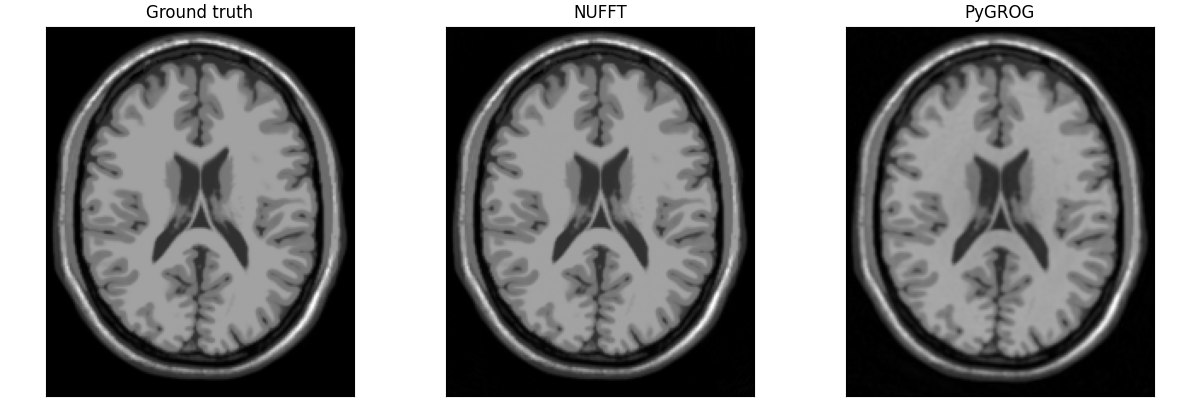
NMSE shortcut  (ret_image=True)    : 1.000e+00
NMSE explicit  (sparse IFFT path)  : 1.000e+00

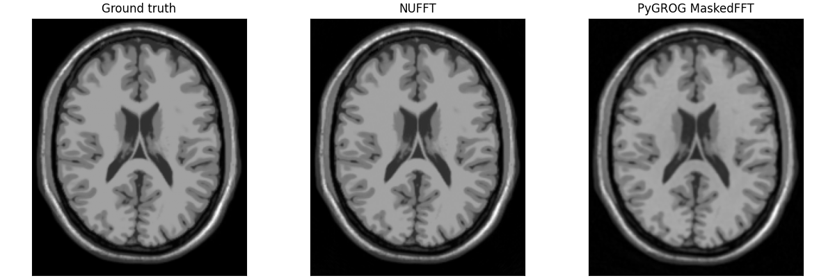
Path 3: Dense-grid path with MaskedFFT

Use interpolate() with grid=True to scatter density-compensated sparse samples onto the full oversampled Cartesian grid, then use MaskedFFT for standard FFT-based reconstruction. The mask and density tensors are passed directly to MaskedFFT, which performs density-compensated reconstruction using masked FFTs instead of NUFFT.

grid_kspace, masked_plan = grog.interpolate(kspace_nc_shaped, grid=True)

print(f"gridded k-space shape : {grid_kspace.shape}")
print(f"masked_plan           : {masked_plan}")
print(f"fraction of mask set  : {masked_plan.mask.float().mean().item():.1%}")

# Build the MaskedFFT operator from the plan — same one-liner as SparseFFT:
#   sparse = grog.interpolate(kspace)
#   op = SparseFFT(plan=grog.plan, smaps=smaps)
#
#   kgrid, plan = grog.interpolate(kspace, grid=True)
#   op = MaskedFFT(plan=plan, smaps=smaps)
masked_fft = MaskedFFT(plan=masked_plan, smaps=smaps)

# Adjoint pass: gridded k-space → SENSE-combined image.
image_masked = np.abs(masked_fft.adjoint(grid_kspace))

nmse_masked = ((image_masked - ref_abs) ** 2).mean() / (ref_abs**2).mean()
print(f"NMSE MaskedFFT path   : {nmse_masked:.3e}")

gridded k-space shape : (16, 272, 227)
masked_plan           : MaskedFFTPlan(grid_shape=(272, 227), image_shape=(217, 181), stack_shape=(), mask=(272, 227), density=(272, 227))
fraction of mask set  : 44.0%
NMSE MaskedFFT path   : 1.000e+00